Large-sample evidence on the impact of unconventional oil and gas development on surface waters by Pietro Bonetti, Christian Leuz, Giovanna Michelon, Aug 20, 2021: Vol. 373, Issue 6557, pp. 896-902. DOI: 10.1126/science.aaz2185
Lightly salted surface waters
Hydraulic fracturing uses a water-based ![]() and sometimes gases, sometimes foamed/gelled gases
and sometimes gases, sometimes foamed/gelled gases![]() mixture to open up tight oil and gas formations. The process is mostly contained, but concerns remain about the potential for surface water contamination. Bonetti et al. found a small increase in certain ions associated with hydraulic fracturing across several locations in the United States (see the Perspective by Hill and Ma). These small increases appeared 90 to 180 days after new wells were put in and suggest some surface water contamination. The magnitude appears small but may require that more attention be paid to monitoring near-well surface waters. Science, aaz2185, this issue p. 896; see also abk3433, p. 853
mixture to open up tight oil and gas formations. The process is mostly contained, but concerns remain about the potential for surface water contamination. Bonetti et al. found a small increase in certain ions associated with hydraulic fracturing across several locations in the United States (see the Perspective by Hill and Ma). These small increases appeared 90 to 180 days after new wells were put in and suggest some surface water contamination. The magnitude appears small but may require that more attention be paid to monitoring near-well surface waters. Science, aaz2185, this issue p. 896; see also abk3433, p. 853
Abstract
The impact of unconventional oil and gas development on water quality is a major environmental concern. We built a large geocoded database that combines surface water measurements with horizontally drilled wells stimulated by hydraulic fracturing (HF) for several shales to examine whether temporal and spatial well variation is associated with anomalous salt concentrations in United States watersheds. We analyzed four ions that could indicate water impact from unconventional development. We found very small concentration increases associated with new HF wells for barium, chloride, and strontium but not bromide. All ions showed larger, but still small-in-magnitude, increases 91 to 180 days after well spudding. Our estimates were most pronounced for wells with larger amounts of produced water, wells located over high-salinity formations, and wells closer and likely upstream from water monitors.
The rise of shale gas and tight oil development has triggered a major public debate about such unconventional development, in which horizontal drilling is combined with hydraulic fracturing (HF). HF is the high-pressure injection of water mixed with chemical additives and propping agents such as sand to create fractures in low-permeability formations, allowing oil or gas to flow. Additives in the HF fluids vary with the geological characteristics of the formation and by operator, but the fluid mix usually contains friction reducers, surfactants, scale inhibitors, biocides, gelling agents, gel breakers, and inorganic acid (1, 2). HF wells produce large amounts of wastewater, which initially consists of flowback of HF fluids but over time increasingly consists of produced water from deep formations. The latter brine is naturally occurring water, into which organic and inorganic constituents from the formation have dissolved, resulting in high salt concentrations (1, 3–5).
Although unconventional oil and gas (O&G) development has been important for energy production (6), we do not fully understand the associated environmental and social risks (7–11). These risks include hydrocarbon emissions, water usage, and pollution, along with potential human and ecological health consequences (7, 10, 12–16). Among these, the impact of unconventional O&G development and HF on water quality remains a key concern (2, 8, 9, 17–20). In the US, one reason for this concern is that HF is exempt from the Underground Injection Control provisions of the Safe Drinking Water Act (8). Around the world, unconventional drilling has either just been introduced, or is being considered, by many countries, with uncertain effects on water quality (16).
The US Environmental Protection Agency (EPA) reviewed and synthetized scientific evidence concerning the impact of HF on US water resources. The final report concluded that HF activities can affect drinking water resources under some circumstances (17), but the report did not identify widespread evidence of contamination. Groundwater studies primarily examine contamination from stray gas or deep formation brines, which could occur because of cementing or casing failures or because of brine migration to shallow aquifers through faults or other preexisting pathways (2, 21, 22). Instances of stray gas contamination have been found in Pennsylvania in connection with shale gas development of the Marcellus Shale (23–29) but not in Arkansas for the Fayetteville Shale (30). Geochemical evidence of gas contamination has also been documented for the Barnett Shale in Texas (24) and the Denver-Julesburg basin in Colorado (31). Studies of brine migration from deep formations, mostly in northeastern Pennsylvania, have provided mixed evidence (23, 32, 33). No evidence of brine contamination of groundwater has been documented for the Fayetteville Shale (30). For Pennsylvania, increases in shale gas–related contaminants have been documented at groundwater intake locations of community water systems that are in close proximity to shale gas wells (18).
For surface water, the evidence is more limited. Instances of contamination have been ascribed primarily to discharges of inadequately treated wastewater, HF fluid leaks, and spills and other mishandling of flowback and produced waters (2, 4, 8, 17, 20, 34, 35). Specifically, increased chloride and bromide concentrations downstream of effluents from wastewater treatment plants have been found in western Pennsylvania up to 2011, when the release of wastewaters from unconventional wells into streams through municipal wastewater treatment plants was not prohibited (2, 4, 36). Further, a high frequency of brine spills in North Dakota has resulted in elevated levels of salts and other contaminants in surface waters up to 4 years after the spills occurred (37). A large-sample statistical examination of the effects of shale gas development activities on surface water in Pennsylvania found higher chloride concentrations downstream of wastewater treatment facilities and an association between gas well density in a watershed and increased total suspended solid (but not chloride) concentrations during the period 2000–2011 (38). The authors of this study suggest that both insufficient wastewater treatment and building infrastructure for unconventional O&G extraction could explain the results. Evidence also exists for barium concentrations in Pennsylvania being higher in areas with unconventional wells than in areas without them, but the authors of this study point out that this evidence cannot be solely ascribed to unconventional wells, as it could also reflect the presence of basin brines or a sulfate decrease in acid rains (39). In sum, prior studies document localized instances of surface water contamination related to unconventional O&G development, with spills and leaks being the most common pathway (20).
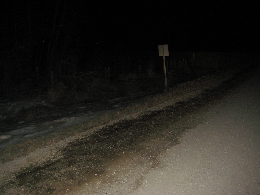
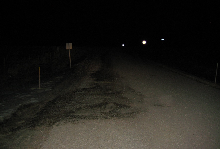
We investigated the potential impact of unconventional O&G development on surface water quality using a large-sample statistical approach. We combined a geocoded database of 46,479 HF wells from 24 shales with 60,783 surface water measurements over 11 years (2006–2016) across 408 watersheds (HUC10s; HUC, hydrologic unit code) with HF activity (Fig. 1, fig. S2, and tables S1 to S3). Our analysis focuses on concentrations of bromide (Br−), chloride (Cl−), barium (Ba), and strontium (Sr) in watersheds exposed to unconventional O&G development. We chose these four ions for the following reasons. First, they are usually found in high concentrations in flowback and produced water from HF wells and hence could indicate surface water impact, if and when it exists (1, 2, 4, 5, 8, 20, 27, 33, 36, 39, 40). Moreover, unlike some organic components of HF fluids, these four ions do not experience biodegradation, and their presence has been measured several years after HF spill events (20, 37). Thus, an analysis of ions is a likely mode of detection (2, 4). Second, many of the water quality concerns associated with HF wastewaters are related to the chemistry of the deep formation brines as well as the salinity in flowback and produced water (8). Third, the four ions are measured in many watersheds with reasonable frequency, which is not the case for other potential signatures of HF wastewater. As high salt concentrations can also occur in surface waters for many natural and anthropogenic reasons, such as brine migration or road deicing ![]() Many states allow frac waste in deicing. Others allow waste to accumulate in landfills then discharged into rivers as landfill leachate. And many jurisdictions – e.g. Alberta, BC, SK, MB – allow companies to dump their drilling waste from frac wells on foodlands (crop and grassland), which also can end up contaminating surface waters via run off, notably after snow melt and storms. Refer below for photos of such waste dumping in Alberta.
Many states allow frac waste in deicing. Others allow waste to accumulate in landfills then discharged into rivers as landfill leachate. And many jurisdictions – e.g. Alberta, BC, SK, MB – allow companies to dump their drilling waste from frac wells on foodlands (crop and grassland), which also can end up contaminating surface waters via run off, notably after snow melt and storms. Refer below for photos of such waste dumping in Alberta.![]() (2, 4, 33, 39), sufficient data is needed to estimate reliable, local, and time-varying baselines for the background ion concentrations.
(2, 4, 33, 39), sufficient data is needed to estimate reliable, local, and time-varying baselines for the background ion concentrations.

We construct these baselines with regression analysis and then exploit temporal and spatial variation in the spudding of HF wells within and across US watersheds to identify anomalous changes in ion concentrations associated with newly spudded HF wells in the same watersheds. Our regression model includes temperature and precipitation control variables as well as an extensive set of fixed effects that construct local and time-varying baselines for background ion concentrations (41, 42). Specifically, our model allows for arbitrary monthly variation in the average background ion concentrations across subbasins (HUC8) and within a given subbasin over time. This flexible regional baseline controls for subbasin differences in water quality, geochemistry, salinity, climate, water body types, or economic activity and also for over-time changes in subbasin concentrations due to seasons, weather patterns and related road deicing, salinization trends, or economic development. Our model also has a local baseline, using each water monitoring station as its own control, which accounts for arbitrary differences in average local ion concentrations. Our model combines these two baselines and the weather control variables to estimate the association between anomalous concentration changes and new HF wells in the same watersheds (42).
Our model explains >80% (in many cases, >90%) of the variation in ion concentrations across watersheds and through time (table S4), suggesting that the model estimates precise baselines for background ion concentrations. We estimated the association between newly spudded HF wells and ion concentrations at the watershed level using a variable that counts the number of HF wells in a watershed at a given point in time (#wellsHUC10). We estimated our regression model for all US watersheds with HF wells and then separately for Pennsylvania, because Pennsylvania accounts for almost 41% of the sample. We found a robust association between new HF wells in a watershed and elevated ion concentrations in its surface waters (Fig. 2 and table S4). For watersheds in Pennsylvania (PA), the coefficients on #wellsHUC10 are positive for all ions and significant for three of them (table S4, column 2, HUC8 model; Br−: 0.00019, P = 0.865; Cl−: 0.00071, P = 0.031; Ba: 0.00038, P = 0.086; Sr: 0.00041, P < 0.001). The lack of significance for Br− could reflect measurement issues (42). For watersheds throughout the US (ALL), the coefficients on #wellsHUC10 are generally comparable to those for Pennsylvania in terms of magnitude and significance, except for Ba, which is rarely measured outside of Pennsylvania and for which results are weaker (Fig. 2). …
To gauge the magnitude of the estimated effects, we multiply each coefficient by the respective sample mean ion concentration and the average number of wells per watershed to obtain the ion concentration increase in the average HUC10 implied by our estimation (HUC10 impact in Fig. 2). With this approach, and focusing on coefficients from the HUC8 specification, we estimated an average increase of Cl− by 1322.44 μg/liter for PA and 2232.55 μg/liter for ALL; Ba by 1.61 μg/liter for PA; and Sr by 5.19 μg/liter for PA and 8.88 μg/liter for ALL (Fig. 2). These magnitudes are very small but need to be interpreted in the context of our analysis. First, the #wellsHUC10 coefficient is by construction a per-well estimate, but this does not imply that each well is associated with a concentration increase, rather it is an average over all wells. Second, by using measurements from all monitors in a given watershed, the estimated well–ion association reflects the average exposure of monitors in the watershed. However, some monitors could be very far away or upstream from wells, in which case they should not be exposed or affected, thus lowering the average. For these reasons, the impact estimates in Fig. 2 are expected to be small; they should increase when the analysis focuses on the most relevant water measurements, as reported below.
We found robust results in different sensitivity analyses (table S5). (i) Estimating separate #wellsHUC10 coefficients for watersheds in and outside of Pennsylvania shows that the findings for Pennsylvania and the other US states are similar. (ii) Estimating separate effects for different time periods shows similar results over time. The coefficients in later periods tend to be smaller but higher in significance, presumably because the frequency of water measurements increases over time. (iii) Our results are similar when the model is estimated over all watersheds within a subregion (including those without HF wells), albeit in some cases slightly weaker, possibly because this specification uses less relevant baselines for the background ion concentrations. (iv) Adding further controls for snow (to account for related discharge of road salts) or for within-watershed seasonality does not alter the findings, suggesting that the monthly subbasin baselines already control for local weather patterns. (v) Our results are also robust to alternative modeling choices, for example, scaling the cumulative number of wells by watershed size, as in (38); estimating the model with weighted least squares (WLS) to give more weight to observations, for which we have more readings to estimate the monthly subbasin baselines; and using alternative transformations to address skewness in ion concentrations.
We also investigated whether the results could be driven by HF-related patterns in the frequency of water monitoring (e.g., more measurements shortly after spud dates or closer to wells). However, we found no evidence that water measurement is systematically related to new wells in a watershed (table S6). We analyzed three other water quality proxies (dissolved oxygen, phosphorus, and fecal coliforms) that are frequently measured but not as indicative of HF-related impacts. Concentration levels of these proxies could be related to other economic activities with water impacts, such as agriculture (43). We used this analysis to gauge how well our model controls for economic activity and other potential confounds. The estimated #wellsHUC10 coefficients for the three analytes are not different from zero (table S7), which contrasts with the results for the ion concentrations we chose for the main analysis (table S4). …
Up to this point, our analysis estimated the long-run association between HF wells and ion concentrations, because we did not restrict the sample and the estimation to a particular period after well spudding. However, concentration increases could be stronger early on and fade over time. Hence, we estimated the association in specific time windows around a new well spud date, allowing us to map out the estimates through time. For this temporal analysis, we modified eq. S1 (see supplementary materials) by replacing #wellsHUC10 with several time-specific well counts, defined for the following time windows measured in days: [−180, −91], [−90, 0], [1, 90], [91, 180], [181, 360], and >360. The coefficients were estimated relative to measurements collected 180 days or more before a new well spudding (table S8). We found increases in ion concentrations 91 to 180 days after the spud date, consistently for all four ions, in Pennsylvania and all US watersheds. In Fig. 3, we plotted the coefficients, estimated over all watersheds, for each window together with the 95% confidence interval. For the [91, 180] window, the well count coefficients are significant for all four ions (Fig. 3 and table S8, panel B; Br−: 0.01095, P = 0.036; Cl−: 0.00401, P = 0.022; Ba: 0.00347, P = 0.017; Sr: 0.00289, P = 0.015). These ion concentration increases in the [91, 180] window are at least one order of magnitude larger than the long-run estimates in table S4 (shown as a red dot in Fig. 3 for comparison). The coefficients for the [91, 180] window (Fig. 3) correspond to an average (short-run) increase of 178.64 μg/liter for Br, 16,014.30 μg/liter for Cl−, 15.46 μg/liter for Ba, and 71.34 μg/liter for Sr per watershed with HF wells. Water measurement is often sparse and, as shown earlier, does not increase around the well spud dates. Thus, most measurements naturally fall into the benchmark period of <−180 days (for which no coefficient is estimated) or in the period beyond 360 days after spudding, which explains why the #wellsHUC10 [>360] coefficients always have the tightest confidence intervals. These coefficients are, as expected, comparable to the long-run estimates from table S4 (red dots in Fig. 3). For all other coefficients, we have far fewer observations, and hence their confidence intervals are wider.
It is useful to interpret the increases in ion concentrations between 91 and 180 days after new well spuddings in the context of the well development and HF process. In our samples, the average time span between the spud date and well completion is 103 days, consistent with (31). Thus, the concentration increases occur after the average HF well is completed and during the early phases of production, when large amounts of flowback and produced water are collected. Although the temporal evidence alone does not identify the exact mechanism for the results, it links elevated concentrations to the unconventional O&G development process.
We conducted two tests that further explore the mechanism by focusing on the role of flowback and produced water at the beginning of production. First, we investigated whether the well–ion associations differ depending on the amount of water a well produces after the spud date. We coded two well count variables at the watershed level: (i) the number of wells with an above-median amount of produced water (#wellsHUC10_High_Prod_Water) and (ii) the number of wells with a below-median amount of produced water (#wellsHUC10_Low_Prod_Water). We defined the medians by subbasin and year to account for regional differences as well as potential changes in HF technology over time. For watersheds where wells generate larger amounts of produced water, we found significant coefficients for Cl− and Sr in all specifications, for Ba in Pennsylvania, and for Br− in one specification (table S9, column 1: Cl−: 0.00057, P = 0.010; Ba: 0.00047, P = 0.064; Sr: 0.00041, P = 0.012; column 2: Cl−: 0.00071, P = 0.031; Ba: 0.00037, P = 0.084; Sr: 0.00041, P < 0.001; column 3: Br− = 0.00035, P = 0.085; Cl−: 0.00057, P = 0.044; Sr: 0.00041, P = 0.002; column 4: Cl−: 0.00058, P = 0.080; Sr: 0.00037, P < 0.001). These coefficients are larger in magnitude than those of their respective low-produced-water counterparts. Admittedly, the amount of produced water is likely correlated with other well and watershed characteristics, and hence differences in coefficient magnitudes between the two groups do not reflect produced water levels alone. Even so, this evidence ties the elevated ion concentrations more closely to HF activity.
Next, we performed an analysis that exploits subbasin variation in the regional geochemistry and the salinity of deep formations (1, 5, 40). The idea was to explore whether the estimated associations are stronger in areas where HF wells are expected to generate produced waters with higher salinity. We used data from the US Geological Survey Produced Waters Geochemical Database and identified subbasins for which produced waters in previous drillings exhibited total dissolved solids (TDS) concentrations above (below) the median, indicating higher (lower) salinity of the deep formations. We created two well count variables at the watershed level: (i) the number of wells in subbasins with an above-median TDS level (#wellsHUC10_High_Salinity) and (ii) the number of wells in subbasins with a below-median TDS level (#wellsHUC10_Low_Salinity). The coefficients in the high-salinity group are positive and larger in magnitude than the coefficients in the low-salinity group (table S10; Br−: 0.00114, P = 0.189; Cl−: 0.00120, P = 0.082; Ba: 0.00064, P = 0.003; Sr: 0.00040, P < 0.001). Thus, the association between new HF wells and ion concentrations is most pronounced in subbasins where deep formations exhibit higher levels of salinity. Importantly, natural brine seepage in high salinity areas cannot explain this result, because the model uses the average concentration levels at the monitoring station as its own control. The result implies a (statistical) link between elevated concentrations and HF wells in areas where produced waters have higher salinity, which is consistent with produced water being part of the mechanism.
As wells can be far from the closest monitor (in our sample, average = 10.3 km and median = 8.2 km), we examined whether the associations between HF wells and ion concentrations are more pronounced when wells and monitors are closer together. However, the sparsity of water measurements makes such distance gradient analyses challenging. We therefore estimate results for different distance bins, [0 to 5 km], [0 to 10 km], and so on up to [0 to 30 km], using either Cl− or pooling observations for all ions in one model. In both cases, we found a negative distance gradient (fig. S5), meaning that the coefficients are largest when we estimated them for wells within 5 km of a monitoring station and then steadily decline when we expanded the widths of the distance bins and included wells that are farther away. Owing to sparse data, our confidence intervals are widest when we include only close-by wells but then become smaller as statistical power increases with the expansion of the distance bins.
To address the data sparsity, and concurrently tighten the analysis, we combined dimensions (such as time, distance, and direction of surface water flows) and then either partitioned or restricted the sample. To partition the sample, we defined watersheds as “high type” when there are relatively (i) more water measurements around new well spuddings, (ii) more monitors in close proximity to new wells, and (iii) more monitors that are likely downstream of new wells (37). We estimated an alternative version of eq. S1, in which we replace #wellsHUC10 with two nonoverlapping well counts, counting the cumulative number of wells spudded in high-type and low-type watersheds, respectively. The associations between HF wells and elevated ion concentrations stem mostly from the high-type watersheds (table S11). This finding is reassuring because it shows that the results come from the types of watersheds that a priori have a higher chance of showing a relation between HF wells and ion concentrations if it exists (e.g., because monitors sit closer to HF wells). …
We also conducted a separate analysis restricting the sample to the most relevant water measurements. We paired all wells and monitoring stations within a watershed so that we could make determinations for each well–monitor pair with respect to time, distance, and direction of water flows. We then restricted the sample to water measurements that are (i) either taken before or up to 360 days after the spud date, (ii) from monitors within a 15-km radius of the well, and (iii) from monitors for which the paired well likely sits upstream, and we estimated eq. S2 using WLS regressions (42). The variable of interest, Post Spud, estimates the average change in the respective ion concentration after a new well spudding, using each well–monitor pair as its own control and after controlling for temperature, precipitation, and monthly variation in background ion concentrations at the subbasin level. We found elevated ion concentrations in the year after new well spuddings (Fig. 4). In the ALL sample, we estimated positive and significant coefficients on Post Spud for Cl−, Ba, and Sr but not for Br− (table S12, panel C; Br−: −0.00577, P = 0.499; Cl−: 0.02044, P = 0.045; Ba: 0.01585, P = 0.048; Sr: 0.02014, P = 0.098). To gauge the magnitude of the estimates, we calculated the 360-day impact on the average watershed, multiplying the respective coefficient by the mean ion concentration and the average number of new wells spudded per year in the average watershed. For the ALL sample, the average 360-day concentration increases are 47,338.29 μg/liter for Cl−, 49.17 μg/liter for Ba, and 282.67 μg/liter for Sr (Fig. 4). These increases are much larger than the long-run increases (Fig. 2) but still well below the EPA maximum contaminant and health advisory levels noted in the Fig. 2 caption. The estimated coefficients are smaller using OLS regressions (table S12, panel D), but even these are still an order of magnitude larger than the respective coefficients for the overall sample (table S4). As a robustness test, we also estimated regressions using observations from “never-treated” monitors that are far away or upstream from any well in the watershed as a control group (table S12, panel E). The results were similar to those in Fig. 4. Notably, the well–monitor pair analysis (Fig. 4 and table S12) showed that estimated well–ion associations strengthened when we focused on the most relevant water measurements.
Our analysis reveals a robust association between new HF wells and elevated concentrations of Cl−, Ba, and Sr in same-watershed surface waters. Our results for Br− are generally weaker and often insignificant. The well–ion association was more pronounced when we estimated it using water measurements from monitors that are close to and likely downstream of wells and from the early phases of production, when wells generate large amounts of flowback and produced water. Although this evidence is based on associations, and as such not causal, the regression analysis controls for a large number of observed and unobserved factors and models background ion concentrations in a flexible and comprehensive manner. Thus, we find it difficult to explain the results by other factors. The confluence of our findings is consistent with unconventional O&G development driving the anomalous surface water ion concentrations identified by our model.
Overall, our evidence complements prior studies on the impacts of unconventional O&G development on water quality [e.g., (2, 8)] and extends studies using a similar large-scale approach for the Marcellus Shale (18, 38). Our statistical approach does not reveal the exact mechanism for the association between new HF wells and concentration increases. There are three potential channels that are particularly relevant in our context (2, 4, 8, 12, 17): (i) on-site accidents; leaks and spills of HF fluids, flowback, and produced water, including those related to pits (overflow, unlined pits, tears in liners); brine trucking; and long-term leaching of soils after spills (4, 12, 20, 35, 37); (ii) direct disposal of untreated wastewater from HF operations (unauthorized or permitted) (4, 8, 12, 35); and (iii) inadequate treatment of wastewater at disposal sites (2, 36, 38). We do not distinguish between these specific channels. However, the consistent increases in ion concentrations shortly after well completion, for wells with large amounts of produced water and for wells located in areas with high-salinity deep formations (Fig. 3 and tables S9 and S10) point to the handling of flowback and produced waters, including leaks and spills, being part of the mechanism for the well–ion association we documented. We explored other explanations and found that our results for HF wells do not reflect the presence of facilities accepting HF wastewater in a watershed (table S13), are not observed for conventional wells (table S14), and are still present when we control for a large number of previously documented spills (table S15). Unknown or undetected spills and leaks could still explain our findings. Independent of the exact mechanism, our results are relevant because we show that the association between unconventional O&G development and elevated ion concentrations extends to many watersheds over several US shales.
We acknowledge that the long-run impact estimates we documented using all watershed monitors are very small in magnitude. However, not all wells are close to surface water and not all monitors are in locations where they could detect an effect. In addition, any impact likely declines over time. Consistent with these arguments, we estimated larger associations when we restricted the analysis to water measurements that are taken within a year of well spudding and from monitoring stations that are closer and likely downstream of wells. But even the 360-day concentration increases implied by these estimates do not exceed EPA limits or health advisory levels for the ions. We also note that water measurements are predominantly from rivers, and hence dilution is another factor to consider when interpreting the magnitude of the associations we estimated.
Our statistical approach was constrained by the ions included in public databases as well as the sparsity of water quality data (2, 4, 20, 27, 41, 44). The former means that we could not examine other analytes in HF fluids or related to unconventional O&G development that are potentially more dangerous than salts. The latter implies that we could not perform more granular analyses that would better identify the mechanism or a causal link. Both limitations of our analysis highlight that investigations of surface water impacts from unconventional O&G development would be greatly facilitated if there were more targeted water measurements of relevant analytes in close proximity to and timed around the development of new HF wells.
Supplementary Materials
science.sciencemag.org/content/373/6557/896/suppl/DC1
Data Description
Research Design
Supplementary Analyses Supporting Statements in the Manuscript
Figs. S1 to S5
Tables S1 to S15
The fracking concern with water quality by Elaine Hill and Lala Ma, Aug 20, 2021, Science, Vol. 373, Issue 6557, pp. 853-854. DOI: 10.1126/science.abk3433
Unconventional oil and gas development (UOGD) has revolutionized resource extraction over the past two and a half decades. Although these methods to recover oil and gas began in the 1980s, only recently have technological innovations in horizontal drilling and hydraulic fracturing (HF) made it financially feasible to extract resources from difficult-to-access rock formations with low permeability (1). These innovations have massively increased the availability of oil and gas resources for consumption, yielding energy cost savings, employment, and income (2). One estimate finds per household benefits to be about 4.9% of income annually (3). Many have cautioned that human and ecological health may be damaged by the negative environmental impacts that come with these benefits. On page 896 of this issue, Bonetti et al. (4) report that UOGD has increased salt concentrations in surface waters across the United States. The findings have broad implications for research and policy going forward.
The investigation of four specific UOGD chemicals was motivated in part by best available data. As Bonetti et al. note, however, there may be other chemicals associated with HF that are potentially more dangerous (5). This highlights the need to expand the set of chemicals measured in the current monitoring system. Moreover, precise measurement of causal effects is dictated by the availability of water monitors, which are spatially sparse. Expanding the geographical scope of water quality surveillance would also improve understanding of the distribution of these effects across regions, different socioeconomic strata, and time. Furthermore, UOGD technology is dynamic. There has been considerable innovation in this industry since UOGD’s mass deployment, which has yielded substantial changes in, for example, the lateral and vertical length of oil and gas wells, the number of wellheads per well pad, whether and how water is reused, and the duration of each stage in the life cycle of a well (6). Notably, these developments affect environmental exposures, and these data are needed to identify the mechanisms of effect. Understanding the exposure pathways at play is necessary for policy to effectively control the environmental damages from these operations.
A looming question also remains regarding whether the water impacts from UOGD translate into health damages or damages on other measures of well-being. Evidence of UOGD water impacts (7) along with studies of the health impacts of drinking water (8, 9) provide indirect evidence that UOGD-related water contamination influences health. Direct evidence is needed. More broadly, continued research in this domain would lend insight into the health benefits of surface water pollution control. A review finds that 67% of US surface water regulations fail a benefit-cost test (10). That these calculations ignore health benefits is among the hypothesized reasons behind the understatement of net benefits.
The findings of Bonetti et al. also suggests a need to rethink regulation. Expanding data collection might be achieved by requiring regulatory agencies to collect and report releases of additional chemicals. Because the magnitude of effects reported by Bonetti et al. are below regulatory thresholds that the US Environmental Protection Agency has for drinking water, tightening the stringency of currently regulated chemicals should be considered. Whether it is advantageous to do so depends on whether the associated chemical emissions yield human and ecological health impacts (information that is not yet known). There are also many UOGD chemicals that are unknown to the public.
All state regulations allow exemptions for trade secrets to incentivize companies to invest in expensive research and development so that they may recoup the benefits of their investment (11).
For regulators, these challenges to setting pollution targets may be overcome by requiring firm disclosure of HF chemicals. Enacting any regulation, however, requires consideration of its cost-effectiveness. At 0.8% of gross domestic product in an average year, water-quality regulation is already among the most expensive environmental policies in the United States (10). Additional regulation may overburden state and local governments. Moreover, firm disclosure of HF fluids may stifle UOGD innovation (12).
It is not an overstatement to say that UOGD has affected all dimensions of life for those in exposed communities (3).
Many of the impacts have lifelong consequences on individual well-being, including future health, education, and labor market outcomes. The mounting evidence on environmental impacts demonstrates a need to quantify and synthesize the associated health and socioeconomic impacts using a common metric. Benefit-cost analysis is particularly useful to facilitate a comprehensive assessment of the consequences of these innovations (13). This type of analysis also requires the clarification of alternative scenarios for comparison and the time frame of consideration. For example, would increasing UOGD regulation cause companies to revert to coal-based energy production (thereby exacerbating pollution) or would it instead spur the transition to a renewables-based future to aid the longer-term battle with climate change? The counterfactual scenario of comparison changes the net-benefit calculation and the optimal policy choice.
It has been more than two decades since the rapid expansion of UOGD, but we are only now beginning to grasp the full scope and extent of the costs associated with these innovations. An understanding of the environmental effects of UOGD is a necessary first step toward a comprehensive assessment of UOGD. Going forward, the mechanisms of impact and their consequences must be clarified to translate this evidence into actionable policy. [References]
Fracking linked to surface water quality for first time in new study by Sharon Udasin, Aug 19, 2021, The Hill
The effects of fracking on nearby water sources may be worse than previously thought, according to a new study that found hydraulic fracturing can alter the composition of surface water and not just groundwater.
The study, published Thursday in Science, is the first to link fracking to small increases in salt concentrations in surface water, particularly during the early stages of production. While the highest salt levels were well below what the Environmental Protection Agency (EPA) considers harmful, researchers identified a robust association between new wells and water quality changes, triggering public health concerns.
“Our work provides the first large-scale sample evidence showing that hydraulic fracturing is related to the quality of nearby surface waters for several U.S. shales,” Christian Leuz, co-author of the study and a professor at the University of Chicago’s Booth School of Business, said in a news release.
The authors analyzed almost 61,000 surface water measurements that had been taken from 2006 to 2016 near about 46,000 hydraulic fracturing wells across 408 watersheds. They investigated the presence of bromide, chloride, strontium and barium, the ions most common in high concentrations in frack “flowback” — the fluid that returns to the surface following fracking operations. Their findings indicated a small but consistent increase in barium, chloride and strontium, but not in bromide.
While Leuz acknowledged that the concentrations might not be alarming at face value, he warned that measurements taken in rivers are susceptible to considerable dilution. In addition, monitors are sometimes situated a couple miles downstream from a fracking site and across entire watersheds — which can be almost as big as a county, he added.
By averaging data from all the wells throughout such expansive spaces, some of which showed impacts and others of which did not, the researchers ended up with these smaller, but still statistically significant, salt concentrations, according to Leuz.
Higher concentrations of barium in drinking water can lead to increases in blood pressure ![]() Tests by Encana/Ovintiv and Alberta Environment showed the barium (and strontium) in my water doubled after Encana illegally frac’d my community’s drinking water aquifers
Tests by Encana/Ovintiv and Alberta Environment showed the barium (and strontium) in my water doubled after Encana illegally frac’d my community’s drinking water aquifers![]() , while chloride can increase water conductivity — the ability of water to conduct electricity — and lead to unpleasant tasting water, as well as potential threats to aquatic life, according to the U.S. Geological Survey.
, while chloride can increase water conductivity — the ability of water to conduct electricity — and lead to unpleasant tasting water, as well as potential threats to aquatic life, according to the U.S. Geological Survey.
Elevated strontium levels can have adverse impacts on bone development.
“They’re not innocuous either,” Leuz told The Hill.
The study identified the highest salt concentrations during the early phases of oil and gas production, when wells generate the most flowback. The researchers also saw higher levels at monitoring stations that were located within 10 miles and downstream from a well, and in measurements taken within a year of the fracking activity.
Co-author Pietro Bonetti, from the University of Navarra in Spain, emphasized the need for more frequent water samples to fully understand the surface water impact, in the news release that accompanied the study. A third co-author, Giovanna Michelon from the University of Bristol in England, called on policymakers to “consider more targeted water measurements” in strategically placed locations.
The three co-authors, who are all economists, became interested in the impacts of hydraulic fracturing on water quality while investigating the ramifications of mandatory chemical disclosure rules that several states — like Wyoming, Pennsylvania and New York — had instituted for hydraulic fracturing operators in 2010. But they first needed to establish a relationship between fracking and surface water quality, which was not yet available, so they implemented their own statistical analysis.
The researchers will conclude a followup study on the effects of disclosure rules in about another month, but Leuz said “the current results suggest that practices became cleaner and had less impact.”
The authors expressed optimism that their statistical approach could be applicable to other fracking chemicals that are even more dangerous than elevated salt levels — but that are rarely included in public databases. For example, recently unearthed documents indicated that the EPA approved the use of fluids that contain toxic forever chemicals.
If the EPA were to conduct regular measurements on such toxic chemicals and make that data available, Leuz said that he and his colleagues could easily run the same statistical analysis on those compounds.
“We could do this for any substance,” he said. “You give me any relevant chemical, and we could apply this approach.” ![]() Hexavalent chromium please. It was found by the regular in the Hamlet of Rosebud’s drinking water supply and chromium went up by a factor of 45 in my water after Encana illegally frac’d our aquifers. (The regulator did not return to test for Hexavalent chromium in my water.) How much of it ended up in the Rosebud River? The Harper (federal) gov’t – good pals with Encana – refused to investigate.
Hexavalent chromium please. It was found by the regular in the Hamlet of Rosebud’s drinking water supply and chromium went up by a factor of 45 in my water after Encana illegally frac’d our aquifers. (The regulator did not return to test for Hexavalent chromium in my water.) How much of it ended up in the Rosebud River? The Harper (federal) gov’t – good pals with Encana – refused to investigate.![]()
Surface Water Vulnerable to Widespread Pollution From Fracking, a New Study Finds, The research suggests that the impacts of the fracking boom may have outrun the science documenting its effects by Bob Berwyn, Aug 20, 2021, Inside Climate News
Fossil fuels don’t just damage the planet by emitting climate-warming greenhouse gases when they are burned. Extracting coal, oil and gas has a huge impact on the surface of the earth, including strip mines the size of cities and offshore oil spills that pollute country-sized swaths of ocean.
Years of research has shown how the fracking boom has contaminated groundwater in some areas. But a study published on Thursday in the journal Science suggests there is also a previously undocumented risk to surface water in streams, rivers and lakes.
After analyzing 11 years of data, including surface water measurements in 408 watersheds and information about more than 40,000 fracking wells, the researchers found a very small but consistent increase in three salt compounds—barium, chloride and strontium—in watersheds with new wells that were fracked. While concentrations of the three elements were elevated, they remained below the levels considered harmful by the EPA.
Such salts are commonly found in water coming from newly fracked wells, making changes in their levels good markers for fracking impacts on surface water, said co-author Christian Leuz, professor of international economics at the University of Chicago. The three economists who did the research specialize in studying the effectiveness of environmental regulations.
Though the impact the researchers detected was small, the data came from diluted water in rivers and streams that were often far from wells, Leuz said, so the concentrations could be higher farther upstream and closer to the fracking operations.
The findings suggest that the rapid pace of “unconventional oil and gas development,” like fracking, may be outrunning scientists’ ability to monitor its impacts on surface water. “Better and more frequent water measurement is needed to fully understand the surface water impact of unconventional oil and gas development,” said economist co-author Pietro Bonetti, with the University of Navarra, Spain.
The researchers said they couldn’t determine human health impacts from the elements for two reasons, Leuz said.
First, “there is not enough public data to analyze potentially more dangerous substances,” he said, and second, ”there are limitations in available water-quality measurements.” Even though some states require fracking companies to disclose chemicals in their fluids, they aren’t always listed in public water monitoring databases, Leuz added.
The 2005 amendment to the Safe Water Drinking Act, known as the Halliburton Loophole, also made tracking harder by exempting hydraulic fracturing fluids from the Safe Drinking Water Act, preventing the EPA from regulating fracking fluids.
A Step Toward Full Accounting of Fossil Fuel Impacts
As the United States seeks to dial back fossil fuel use, accurate environmental data is important for policy discussions about topics like carbon pricing, as analysts try to present a full accounting of how much fossil fuels cost, said co-author Giovanna Michelon, who researches sustainability accounting at the University of Bristol.
The study, she said, was started to determine if regulations requiring companies to disclose the contents of their fracking fluids had an impact on water quality during the fracking boom, when tens of thousands of wells were drilled in Pennsylvania and New York, and through a vast swath of the West, from Oklahoma and Texas through New Mexico, Colorado, Utah, Wyoming, Montana and North Dakota.
Around 2010, many states started regulating fracking which, along with technologies that allowed horizontal drilling for miles underground, drove the boom in “unconventional oil and gas development” and obliged companies to disclose more environmental information related to fracking, including the chemicals in their fluids and details on wastewater management.
“We wanted to see if the mandatory disclosure made their operations cleaner,” Michelon said. But as the researchers started collecting information on new wells and water quality, they realized that there wasn’t enough data to show that link, she added.

… Early research on fracking impacts was mostly on groundwater contamination, but in 2016, the EPA published a report with a “more complete record of localized evidence,” that found the potential for surface water pollution under certain circumstances, Michelon said.
… “There are three potential channels that may be related to our results, but we are unable to discriminate or distinguish between them,” Michelon said. They include on-site spills and leakage, a long-term slow escape of water called leaching and improper disposal or treatment of wastewater, including “direct disposal of untreated wastewater,” which may be done illegally or permitted by insufficient regulation, she said. ![]() What good are regulations? Companies everywhere usually just ignore them, and regulators/courts enable them.
What good are regulations? Companies everywhere usually just ignore them, and regulators/courts enable them.![]()
The Critical Zone
Sue Brantley, a geochemist at Penn State, studies water in what she calls the critical zone—from treetops down to groundwater—because it’s where nearly all human interaction with water happens. For her, the new study partly answers a long-standing question.
“Is fracking affecting water in the critical zone to the extent that we need to do something about it?” asked Brantley, who was not a study author, but reviewed a draft of the report. The advanced statistical analysis used by the research team produced results that correlated fracking with changes to water chemistry. “I don’t think anyone has ever really seen that before,” she said.
“Those are the kind of numbers that a health expert needs to start doing assessments,” she said, adding that other studies have shown health impacts like babies with lower birth weights and higher rates of asthma in areas with fracked wells.
And even though the increases detected by the study are small, the findings hint at the looming problem represented by the massive amounts of tainted water produced by fracking.
“We’re drilling a lot of deep holes into permeable rock, and those are conduits up into the critical zone—straws down out of our critical zone,” she said. “They can bring up elements and compounds that are potentially dangerous. You’re bringing up very concentrated brine, and when you look at how much brine is being collected from all the wells around the country, it raises concerns.” …

Refer also to:
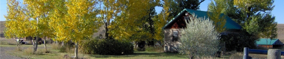
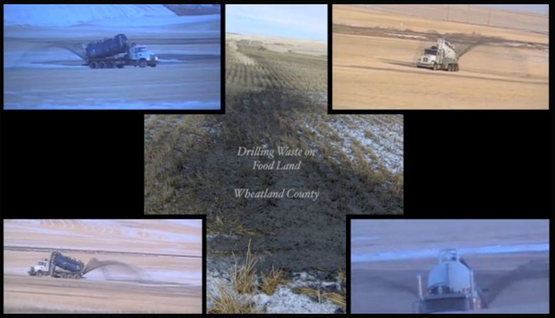
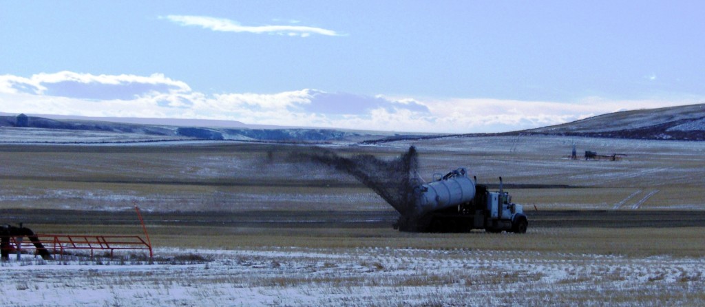
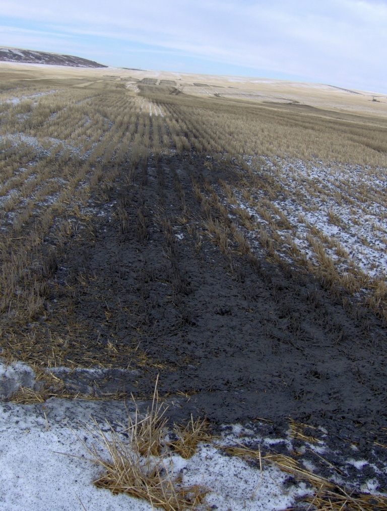
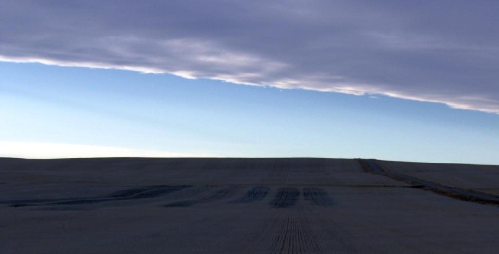
Encana dumping drilling waste from wells later frac’d on foodland just outside my community, Rosebud Alberta, and just uphill from the Rosebud River and drainages/creeks running into it:
2011:
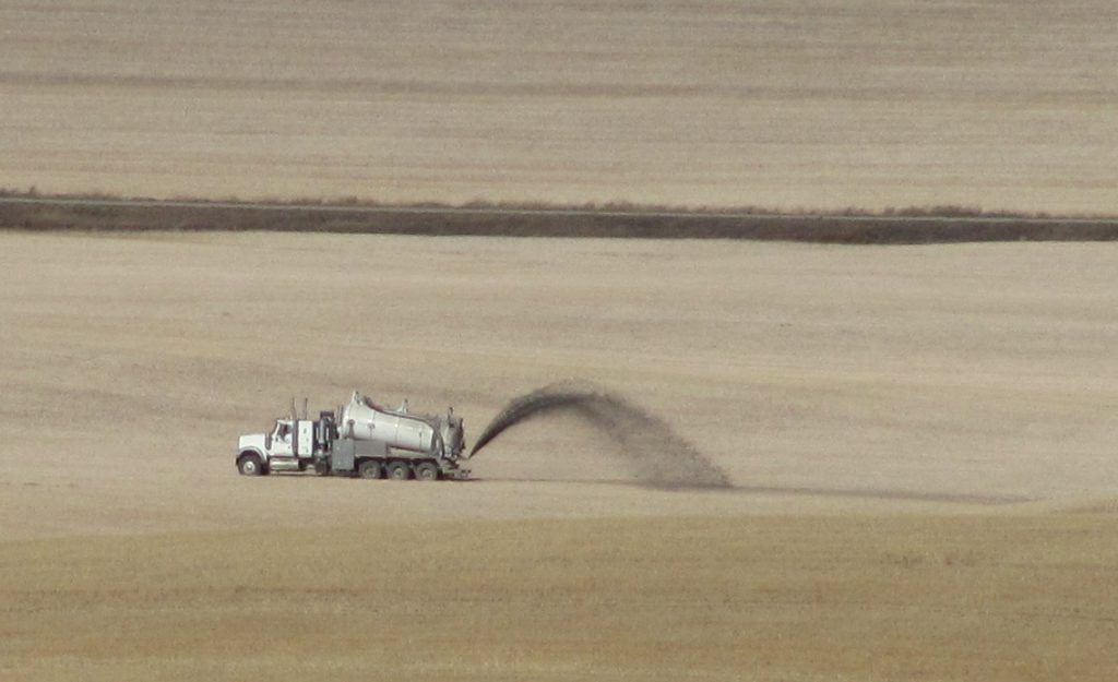
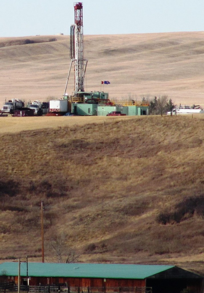
Above waste came from this well being drilled in photo below. I watched the trucks load up the waste and dump about nearby:
My water well is in the barn with the green metal roof in above photo. The old Rosebud River bed meanders through my land, just behind the barn:
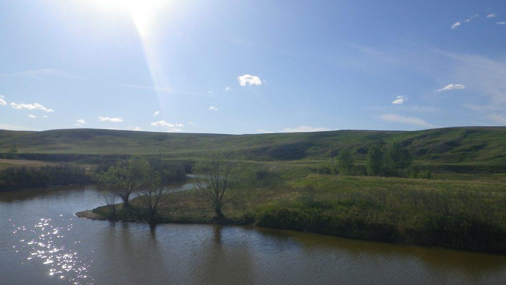
The old Rosebud River meandering through my land
2012 (Encana dumped their waste in the same location. This year, company contractors observed me observing and filming them, and thereafter Encana chose locations not visible from public roads to do their dumping):
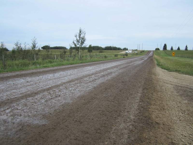
Another company dumping their waste in Alberta NW of Calgary:

Some companies dump their waste on Alberta public roads while the regulator is busy looking the other way or doing the hanky panky:
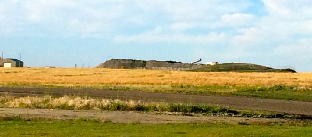
Oilfield waste piling high near Didsbury, Alberta, another potential source of contamination into the Rosebud River:
2013: Integrated Water Technologies Inc. seeks to use fracking waste on roads, sidewalks
2013: Sewage Plants Struggle To Treat Wastewater Produced By Fracking Operations
2013: Trio charged with illegal frack water dumping
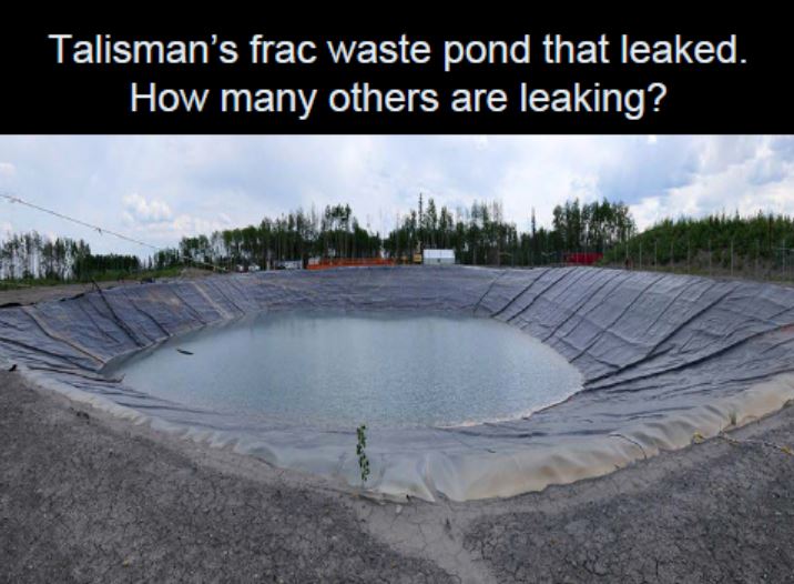
2013: Talisman frackwater pit in NE BC leaked for months, kept from public
2014: GreenHunter Could Store Toxic Water Next to Ohio River, Concern Grows Following Spill In Kanawha
2016: THREE NEW STUDIES: FRAC WASTE CONTAMINATES WATER AND SOIL, SOME FOR THOUSANDS OF YEARS

Encana/Ovintiv dumping its waste on foodland at Rosebud, Alberta
Endless more posts on this website and elsewhere.